

1. Overview
In this tutorial, we’re going to study the differences between classification and clustering techniques for machine learning.
We’ll first start by describing the ideas behind both methodologies, and the advantages that they individually carry. Then, we’ll list their primary techniques and usages.
We’ll also make a checklist for determining which category of algorithms to use when addressing new tasks.
At the end of this tutorial, we’ll understand what’s the function of classification and clustering techniques, and what are their typical usage cases.
2. Classification
2.1. Introduction to Classification
Both classification and clustering are common techniques for performing data mining on datasets. While a skillful data scientist is proficient in both, they’re not however equally suitable for solving all problems. As a consequence, it’s therefore important to understand their specific advantages and limitations.
We’ll start with the classification first. After briefly discussing the idea of classification in general, we’ll then see what methods we can use to implement it for practical tasks.
Classification problems are a category of problems that relate to supervised learning in machine learning. It corresponds, in brief, to assigning labels to a series of observations. As we discussed in our article on labeled data, classification in the real-world is possible only when we have prior knowledge of what the labels represent semantically.
While the problem of classification can, in itself, be described in exclusively mathematical notation, the development of a machine learning system for deployment into the real world requires us to consider the larger systems in which our product will be embedded. This, in turn, requires mapping the labels into some kind of real-world semantic categories.
Classification also conveys to the idea that, in general, we may want to partition the world into discrete regions or compartments. These regions tend to be non-overlapping, even though the formulation of overlapping labels is possible through hierarchical or multi-label classification. Even when the regions overlap, though, the labels themselves don’t.
Classification is, therefore, the problem of assigning discrete labels to things or, alternatively, to regions.
2.2. Classification in Short
The underlying hypotheses of classification are the following:
- There are discrete and distinct classes
- Observations belong to or are affiliated with classes
- There’s a function which models the process of affiliating an observation to its class
- This function can be learned on a training dataset and generalizes well over previously unseen data
These hypotheses are all equally important. If one of them is violated, then classification wouldn’t work for a given problem.
2.3. What Do These Hypotheses Mean?
The first hypothesis is simple to understand, and it just means that classes aren’t continuous values. If they were, we’d be solving a regression, not a classification problem.
With regard to the second hypothesis, we can use the following intuitive example. Let’s imagine that somebody gives us the task to classify these polygons:
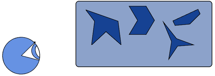
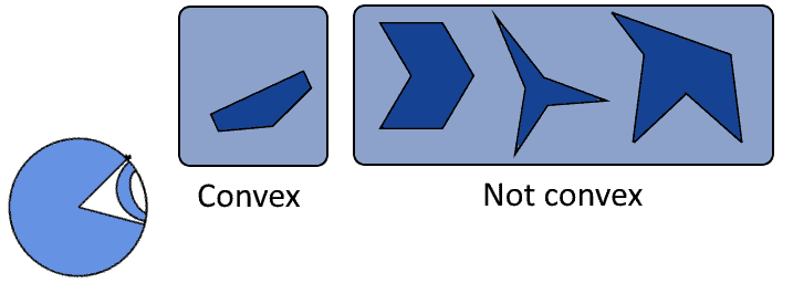
Unless the task giver specifies a typology according to which we should do classification, then classification is impossible. If they, however, told us to divide them into convex and non-convex, then classification would be possible again:
We couldn’t however classify the same polygons according to the categories  , for example.
With regard to the third hypothesis, this is important because classification doesn’t only concern machine learning. As is the case for the recognition of objects by humans in satellite images, it’s possible to conduct object recognition even with human understanding alone. In that case, the process of classification can be modeled as a workflow that involves a human as one of its elements, but can’t be properly modeled as a mathematical decision function:

With regard to the last hypothesis, we can use, instead, this example. Let’s imagine that our task is to identify objects in images, but that we’re provided with a dataset containing only vehicles:
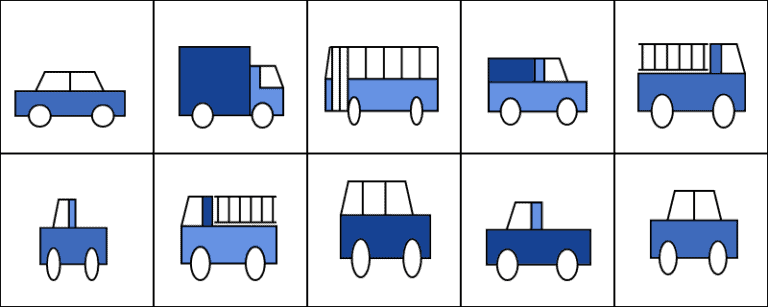
No matter what algorithm we’ll use, the identification of any objects other than vehicles is impossible. We can analogously say that, by using this dataset,  . If we want to identify, say, bicycles, then this sample dataset is inappropriate, for violation of the fourth hypothesis.
3. Common Methods for Classification
3.1. Logistic Regression
The methods for classification all consist of the learning of a function that allows, given a feature vector  , to assign a label
  corresponding to one of the labels in a training dataset. We’re now going to see in order some of the primary methods, and examples of their application.
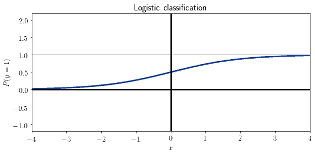
Logistic regression is one of the most simple methods for classification. It simulates the decision to assign classes to observations, by modeling the process as the determination of a probability  continuously distributed in the interval
  . Logistic regression is particularly common as a classification method because its optimization function is treatable with gradient descent. This, in turn, guarantees that the model can be optimized procedurally:
3.2. Naive Bayesian
Naive Bayesian classifiers are the typical tool for building simple classification systems for feature vectors with strong linear independence between their components. Ironically, it’s frequently used for features like texts that certainly have a strong linear dependence.
It’s however particularly useful in contexts where we have no indication of the general shape of the classification function, and when we can assume that the training dataset is well representative of the real-world data that the machine learning system would retrieve.
The foundation of Naive Bayesian classification is Bayes’ famous theorem, which calculates the probability  of given the feature
  of the feature vector , as:

3.3. Convolutional Neural Networks
Neural networks, and in particular convolutional neural networks, help solve the task of classification for datasets where the features have a strong linear dependence on one another. The way they work is by reducing the dimensionality of the input to the classifier, such that the classification task can take place without excessive requirements in terms of computational power and time.
Several activation functions exist for convolutional neural networks. Intermediate layers normally use ReLU or Dropout functions, while the classification layer generally uses softmax.
3.4. Support Vector Machines
Another common algorithm for classification is the support vector machine, also known as support vector classifier in this context. This algorithm works by identifying a separation hyperplane that best segregates observations belonging to different classes:
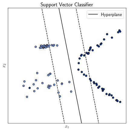
Support vector machines are similar to neural networks insofar as they’re both parametric, but there are otherwise several differences between them. They tend to be significantly more rapid to train than neural networks, but tend to be slower in computing the result of their predictions.
4. Usages of Classification
The usages for classification depend on the data types that we process with it. The most common data types are images, videos, texts, and audio signals.
Some usages of classification with these types of data sources are:
- In image processing, classification allows us to recognize objects such as characters in an image
- In video processing, classification can let us identify the class or topic to which a given video relates
- For text processing, classification lets us detect spam in emails and filter them out accordingly
- For audio processing, we can use classification to automatically detect words in the human speech
There are also some less common types of data, that still use classification methods for the solution of some particular problems:
- In weather control, the forecast of weather can take place with classifiers trained on data from weather stations
- In systems maintenance, the identification of faulty components can occur thanks to appropriately trained classifiers
- For astronomy, supervised learning can help detect planets out of the solar system on the basis of readings from the Kepler telescope
- For mining and resource extraction, classification can identify the probability to find ore deposit on the basis of GIS and geological data
- In neurology, classifiers can help fine-tune EEG models for brain-machine and brain-to-brain interfaces
Many more applications of supervised learning and classifications exist. As a general rule, if a problem can be formalized in a way that respects the four hypotheses we identified above, then that problem can be tackled as a classification problem.
5. Clustering
5.1. An Introduction to Clustering
The other approach to machine learning, the alternative to supervised learning, is unsupervised learning. Unsupervised learning comprises a class of algorithms that handle unlabeled data; that is, data on which we add no prior knowledge about its class affiliation.
One of the most important groups of algorithms for unsupervised learning is clustering, which consists in the algorithmic identification of groups of observations in a dataset, that are similar to one another according to some kind of metric.
We mentioned in the section on the introduction to the classification that labels, there, have to be aprioristically determined and discrete. Clusters, though, don’t have to be pre-determined, and it’s, in fact, possible to cluster into an unknown number of them.
The most simple way to understand clustering is to refer to it in terms of feature spaces. A feature space is a space in which all observations in a dataset lie. We can conceptualize it in two dimensions, by imagining it as a Cartesian plane:
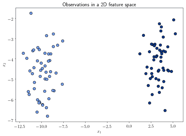
We can see from the image above that the observations all lie within that feature space. However, not all of them lie in the same region of that space. We can, in fact, identify some that are significantly close to one another, while far away from groups of others:
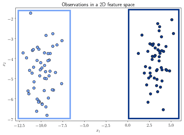
The problem of determining groups of observations that belong together, by means of their similarity, takes the name of clustering.
5.2. Clustering in Short
As we did for classification, we can now list the hypotheses required to apply clustering to a problem. There are only two that are particularly important:
- All observations lie in the same feature space, which is always verified if the observations belong to the same dataset
- There must be some metric according to which we measure similarities between observations in that space
If the feature space is a vector space, as we assume it to be, then the metric certainly exists.
These hypotheses are significantly less restrictive than the ones needed for classification. We can say, in this sense, that clustering requires limited prior knowledge on the nature of the phenomenon that we’re studying, with comparison to classification. Keep in mind, however, that specific algorithms may have additional hypotheses on the expected distribution of clusters, and that these should be factored, too, when choosing a specific algorithm.
Clustering is often helpful in hypothesis formulation and finds application in the automation of that task, too. This means that it’s mostly a maker, rather than a subject, of hypotheses.
6. Common Methods for Clustering
6.1. K-Means
We can now study the specific techniques that we can use to conduct clustering on a dataset. For the purpose of displaying how different techniques may lead to different results, we’ll always refer to the same dataset, the famous Iris dataset:
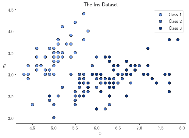
Notice that the Iris dataset has classes, that are typically used for supervised learning. However, we can simply ignore the class labels and do clustering instead. We can refer back to the image above to see how the various clustering techniques compare to the class distribution, if interested.
The first technique that we study is K-Means, which is also the most frequently encountered. K-Means is a parametric algorithm, that requires the prior identification of the number of clusters to identify. It works by identifying the points in the feature space that minimize the variance in the distance with all observations that are closest to them:
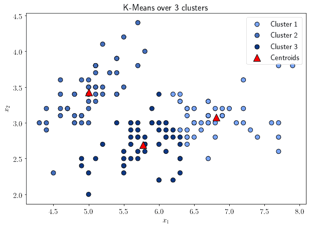
These points take the name of “centroids” of the cluster. The formula that computes K-Means over a dataset with  observations
  is this:

This works by identifying the mean values  , one per cluster, that minimizes the square of the distance with each observations belonging to that cluster.
6.2. DBSCAN
DBSCAN is an algorithm that takes a different approach to cluster analysis, by considering not distances but rather density of points in the feature space. Its underlying hypothesis is that a region with a high-density of observations is always surrounded by a region with low-density. This is, of course, not universally valid, and we need to take this into account when selecting DBSCAN for our applications.
The high-density region also takes the name of “neighborhood”. DBSCAN is then parameterized by two values: one, that indicates the minimum number of samples in a high-density neighborhood; and the other, that indicates the maximum distance that observations belonging to a neighborhood can have with respect to that neighborhood:
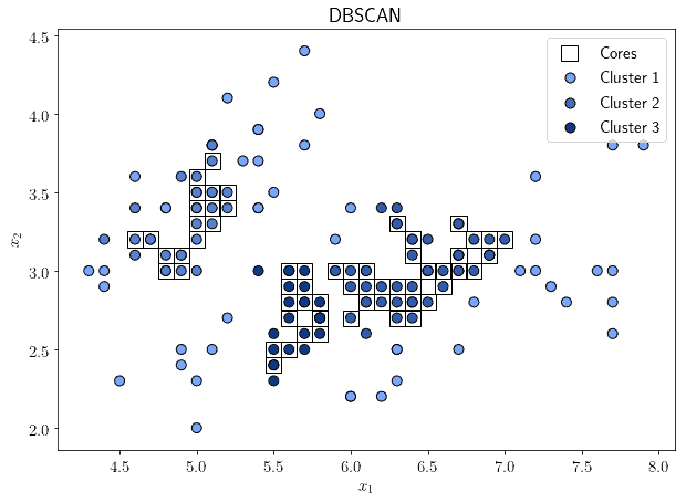
The “cores” are the samples located in a high-density neighborhood, while the other samples are all located in low-density regions.
6.3. Spectral Clustering
Spectral clustering is an algorithm that works by first extracting the affinity matrix of a dataset, and then by computing another clusterization algorithm, such as K-Means, on the eigenvectors of the normalized version of that matrix:
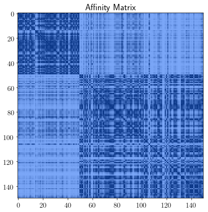
The clusters that are identified in the low-dimensional space are then projected back to the original feature spaces, and cluster affiliation is assigned accordingly:
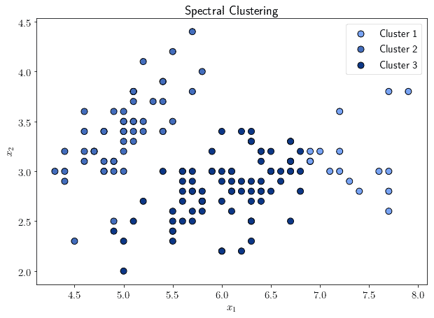
One major advantage of spectral clustering is that, for very sparse affinity matrices, it tends to outperform other clustering algorithms in computational speed. It tends to underperform, however, if the number of clusters is significantly high.
6.4. Mean Shift
Another centroid-based algorithm is the mean shift, which works by iteratively attempting to identify cluster centroids that are placed as close as possible to the ideal mean of the points in a region. This takes place by first placing the centroids randomly, and then updating their position so that they shift towards the mean:
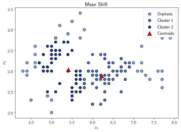
The algorithm identifies as clusters all observations that comprise a region of smooth density around the centroids. Those observations that lie outside of all clusters take the name of orphans. One of the advantages of a mean shift over other forms of clustering algorithms is that it allows clustering only the subset of all observations that are within the same region but doesn’t require to consider them all.
6.5. Affinity Propagation
Affinity propagation works by constructing a graph comprised of the observations contained in the dataset. Then the algorithm simulates the sending of messages between the pairs of points in the graph, and then determines which points represent most closely the others:
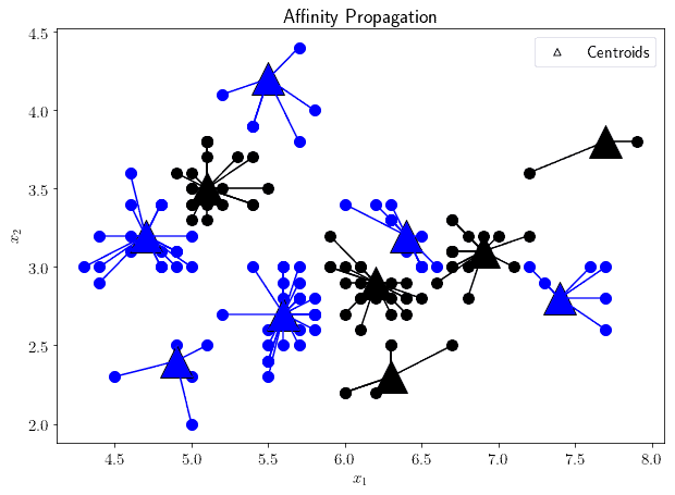
The primary advantage of affinity propagation is that it doesn’t require the apriori determination of the number of clusters in the dataset. Instead, the algorithm is parameterized according to a value called preference, which indicates the likelihood that a particular observation may become representative of the others.
Another advantage of affinity propagation is that it continues to perform well when the clusters contain a significantly different number of observations, where other algorithms may end up suppressing the smaller clusters or integrating them into the larger ones.
7. Usages of Clustering
7.1. Common Usages
We can now see some common usages of clustering in practical applications. As was the case for classification, the nature of the data that we’re treating with clustering affects the type of benefit that we may receive:
- For texts, clustering can help identifying documents characterized by the highest similarity, which is useful to detect plagiarism
- For audio signals and, in particular, for speech processing, clustering allows the identification of speeches that belong to the same dialect in a language
- When working with images, clustering lets us identify images that are similar to one another, short of a rotational, scaling, or translational transformation
- For videos, and in particular, for the tracking of faces, we can use clustering to detect the parts of images that contain the same face across multiple frames
7.2. Less Common Usages
There are however less common data types on which we can still use clustering:
- In geospatial imagery, we can identify elongated regions such as road by means of cluster analysis
- In autonomous driving, it has been proposed that the clustering of autonomous vehicles and the identification of cluster-level rules for behavior can help ease traffic
- For the survey of the fish population in fisheries, clustering can help increase the representativeness of the sampling process and avoid bias
- In social network analysis, clustering is commonly used to identify communities of practice within a larger social organization
One last thing to mention is that sometimes clustering and classification can be integrated into a single sequential process. The common example is the identification of groups of comments among the reviews or complaints on a website; which is a task that, when handled for the first time by a new website, can’t rely on the prior identification of labels.
8. The Checklist
We can now formulate a checklist that allows us to determine what category of algorithms we should use when faced with a new dataset. If we include the prior hypotheses to each category, as we identified them in the previous sections, we’d obtain this table:

9. Conclusions
In this article, we studied the differences between classification and clustering.
We also listed the prior hypotheses that each class of machine learning algorithms embeds. In doing so, we could formulate a checklist against which we can compare our dataset.
This, in turn, lets us determine whether we should use classification or clustering for a given task, according to its characteristics.