

1. Introduction
When training a Machine Learning (ML) model, we should define a set of hyperparameters to achieve high accuracy in the test set.
These parameters include learning rate, weight decay, number of layers, and batch size, to cite a few.
In this tutorial, we’ll discuss the main differences between using the whole dataset as a batch to update the model and using a mini-batch.
Finally, we’ll illustrate how to implement different gradient descent approaches using TensorFlow. First, however, let’s understand the basics of when, how, and why we should update the model.
2. Gradient Descent Calculation
Usually, a Deep Learning problem can be seen as an optimization problem. Our goal is to either maximize or minimize some functions. The minimization problem is more common in ML, and we refer to this function as a loss function.
How can we reach the minimum point of a loss function?
The most common approach is to use gradient descent. We use the derivative of the function at some point to check if the tendency is to increase or decrease its value.
We can easily see how gradient descent works with a quadratic function:
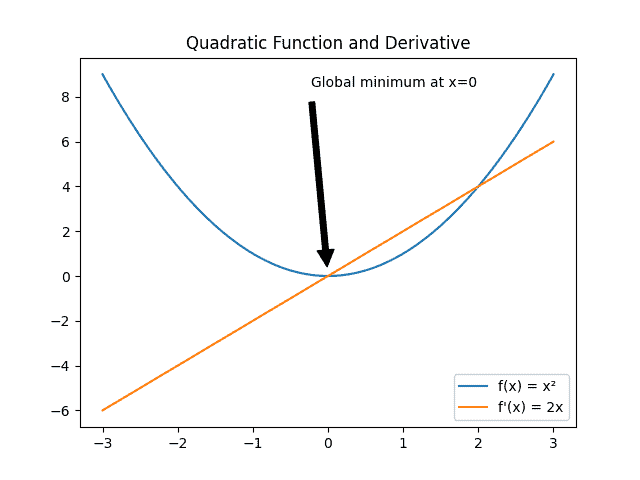
Let’s suppose we want to find the minimum of  .
.
We randomly start at the point  , calculating the derivative at this value:
(1) 
From this point, we analyze the signal of the result. In this case, the derivative is negative, so we should take a step on the opposite side, in the positive direction.
If we take a step equal to  , we’ll reach the point
  , and once again we calculate the derivative:
(2) 
Now the derivative is greater than zero, so we take a step in the negative direction. If we take enough steps with the right size, we’ll reach the global minimum  .
.
If we take a large step, we might never find the minimum because we’d bounce from one point to another. Conversely, if we take really small steps, the process will take a lot of time.
The learning rate will define the size of the step we use to update the values of the model.
3. Batch Size
We can take a step in the gradient descent, and update the parameters in different ways. The chosen approach will dramatically define the performance and convergence of the model.
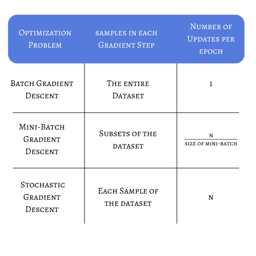
Before we move on, it’s essential to highlight the concepts of epoch and batch.
After our entire training set is seen by the model, we say that one epoch is finished.
During the training, we can update the weights and gradient after a subset of the whole training set is computed by the model. We call this a subset batch or mini-batch.
One of the most common problems we face when training a neural network is that the loss function might have some points of local minima that can mislead us that the model achieved its best possible state:
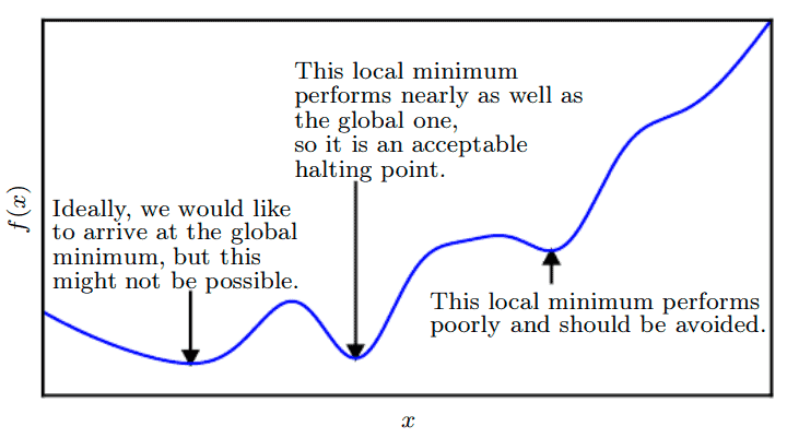
We’ll address how different batch sizes will affect the training process, and sometimes prevent our model from getting stuck in a local minimum or flat region, known as a saddle point.
3.1. Batch Gradient Descent
The most straightforward approach we have is Batch Gradient Descent or Gradient Descent (GD). In this approach, we’ll compute the gradient only after the whole dataset is used in training.
One of the main concerns regarding this strategy is that if our training set has hundreds of thousands of samples, we’ll need an enormous amount of memory. This is because we’ll need to accumulate the errors for each sample until the whole dataset is evaluated. Then the parameters will be updated, and the gradient descent will terminate one iteration.
With this optimization strategy, we’ll update the model only a few times. As a result, the loss function will be more stable, with less noise. However, there is one drawback. For non-convex problems with several local minima, we might get stuck in a saddle point too early and finish the training with parameters far from the desired performance.
3.2. Mini-Batch Gradient Descent
In mini-batch GD, we use a subset of the dataset to take another step in the learning process. Therefore, our mini-batch can have a value greater than one, and less than the size of the complete training set.
Now, instead of waiting for the model to compute the whole dataset, we’re able to update its parameters more frequently. This reduces the risk of getting stuck at a local minimum, since different batches will be considered at each iteration, granting a robust convergence.
Although we don’t need to store the errors for the whole dataset in the memory, we still need to accumulate the sample errors to update the gradient after all mini-batches are evaluated.
3.3. Stochastic Gradient Descent
When we use Stochastic Gradient Descent (SGD), the parameters are updated after each sample of the dataset is evaluated in the training phase. SGD can be seen as a mini-batch GD with a size of one.
This approach is considered significantly noisy since the direction indicated by one sample might differ from the direction of the other samples. The problem is that our model can easily jump around, having different variances across all epochs.
In some ML applications, we’ll have complex neural networks with a non-convex problem; for these scenarios, we’ll need to explore the space of the loss function.
In this way, we’ll escape from a bad local optimum, and be more likely to find the global optimum.
One of the main advantages of SGD is having an early indication of the model’s performance since the parameters are constantly updated.
However, models with high complexity and large training datasets will take a lot of time to converge, turning the SGD into a very expensive optimization strategy.
4. TensorFlow Example
In this section, we’ll use a real-world example to illustrate the impact of different batch sizes in the training of a neural network.
Before we look at the example, let’s summarize the main differences between each strategy, considering a dataset with N samples:
For this example, we’ll use the TensorFlow model of a convolutional neural network to recognize handwritten digits. Our training set has 54000 samples of 24×24 images. The validation set used to adjust the parameters has 6000 samples, and the test set for final accuracy has 10000 samples.
We’ll use three different batch sizes. In the first scenario, we’ll use a batch size equal to 27000. Ideally, we should use a batch size of 54000 to simulate the batch size, but due to memory limitations, we’ll restrict this value.
For the mini-batch case, we’ll use 128 images per iteration. Lastly, for the SGD, we’ll define a batch with a size equal to one.
To reproduce this example, it’s only necessary to adjust the batch size variable when the function fit is called:
model.fit(x_train, y_train, batch_size=batch_size, epochs=epochs, validation_split=0.1)We can easily see how SGD and mini-batch outperform Batch Gradient Descent for the used dataset:
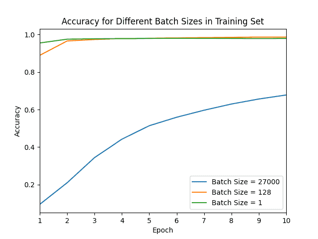
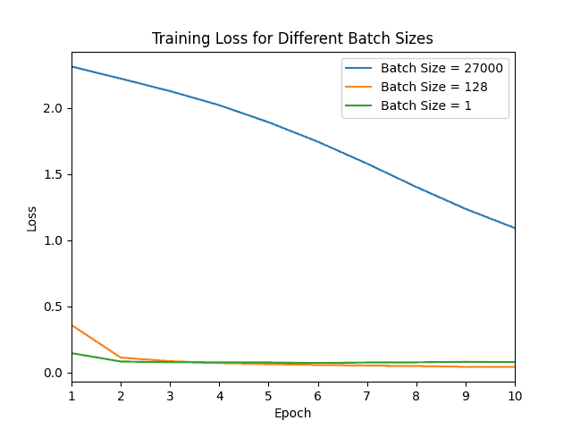
With a batch size of 27000, we obtained the greatest loss and smallest accuracy after ten epochs. This shows the effect of using half of a dataset to compute only one update in the weights.
From the accuracy curve, we see that after two epochs, our model is already near the maximum accuracy for mini-batch and SGD. This happens because the samples used for training, although not equal, are very similar.
This redundancy makes Batch GD perform poorly when time constraints are also considered.
5. Conclusion
There’s no strict rule to define which batch size we should use in our training. This is a hyperparameter we should tune.
We can follow general guidelines to adjust it to achieve a satisfactory model.
If we know beforehand that our problem involves a convex loss function, then batch gradient descent might be a good fit. It’s also helpful because sometimes it finds the minimum point in a reasonable time.
Conversely, if our dataset has millions of samples and our loss function will most likely have many local minima, we should consider using a mini-batch or SGD optimization.
In this way, instead of waiting for thousands of samples to be evaluated, we’ll have some indication about how our model is performing after only a few hundred iterations.