Hidden Markov Models vs. Conditional Random Fields

1. Overview

Hidden Markov Models (HMMs) and Conditional Random Fields (CRFs) belong to the family of graphical models in machine learning.

In this tutorial, we’ll cover their definitions, similarities, and differences.

2. Hidden Markov Models (HMMs)

Let’s imagine that we have an English sentence like Math is the language of nature. We want to label each word with its part of speech. That way, we get a graph:

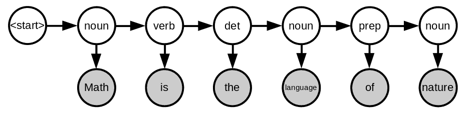
example of first-order hidden Markov model

Let’s see what each color and arrow represent. The sentence is our observed data (shown in gray circles) and the labels are the hidden information we want to extract (shown in white circles). In addition, each word depends on its label and each label depends on the previous label.

This graph represents a first-order hidden Markov model which belongs to the family of Bayesian networks. The reason why we call it “first-order” is that each hidden variable depends only on the previous one. We can extend it to a higher-order model by conditioning the hidden variables on more than one predecessor.

The general first-order HMM graph for any sequence is similar to that of our example:

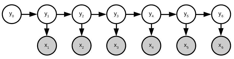
We can assign probabilities to each arrow and model the occurrence of such a sequence using the product of these probabilities:

$p(\textbf{x},\textbf{y}) = \prod_{i=0}^{i=n} p(x_i|y_i)p(y_i|y_{i-1})$

where $\textbf{x}$ and $\textbf{y}$ are the sequence and the array of its labels. The $p(x_i|y_i)$ are emission probabilities and the $p(y_i|y_{i-1})$ are transition probabilities. The former is the set of probabilities for each observation given its corresponding state while the latter is the probability of a state given its preceding state. Since an HMM models the joint probability of $\textbf{x}$ and $\textbf{y}$ , it’s a generative model.

2.1. Example

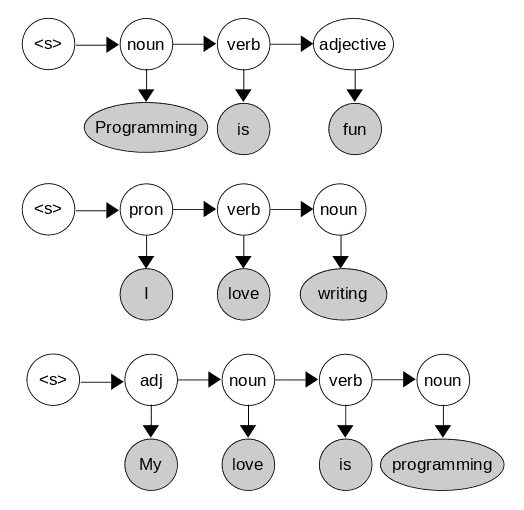
Let’s imagine we want to tag the words in the sentence I love programming. From our training data, we can learn the emission and transition probabilities by counting. For instance, let’s imagine that the training data consists of three sentences:

From there, we calculate the emission probabilities:

and the transition probabilites:

To find the optimal labels, we can go over all the combinations of states and observations to find the sequence that has the maximum probability. For our example, the best sequence is:

$p(\text{pron}|\texttt{start}) \times p(\text{I}|\text{pron}) \times p(\text{verb}|\text{pron}) \times p(\text{love}|\text{verb}) \times p(\text{noun}|\text{verb}) \times p(\text{programming}|\text{noun}) =$

$0.33 \times 1 \times 1 \times 0.33 \times 0.67 \times 0.5 = 0.0364815$

Given that our example was a small one with only a couple of words and parts of speech, it’s easy to enumerate all the possible combinations. However, this can become extremely difficult to do in more complex and longer sentences. For them, we use inference algorithms such as Viterbi or Forward-backward.

3. Conditional Random Fields (CRFs)

A CRF is a graphical models of $p(y|x)$ instead of $p(x, y)$ . This makes it a discriminative model since we only want to model the hidden variables conditioned on the observations. As a result, we do not care about their marginal distributions.

3.1. Feature Functions

CRFs are undirected graphical models, for which we define features (i.e., feature functions) manually. Simply put, feature functions are descriptions of words depending on their position in the sequence and their surrounding words. For example, “The word is a question mark and the first word of the sequence is a verb.”, “This word is a noun and the previous word is a noun”, or “This is a pronoun and the next word is a verb”. After selecting the feature functions, we find their weights by training the CRF.

Here’s a schematic representation of a CRF:

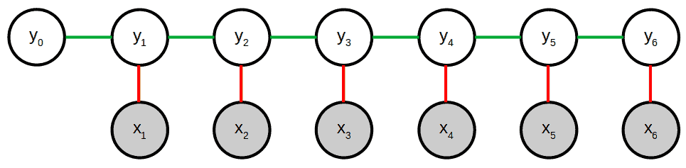
There are two types of feature functions: the state and transition functions. State functions (red in the above graph) represent the connection between hidden variables and the observed ones. Transition functions (green) do the same for the hidden states themselves. We can define an arbitrary number of feature functions depending on the specific task we want to perform.

For instance, for our previous example of POS tagging, one feature can be whether a word and its predecessor are of the same type. Another one could be whether the current word is the end of the sequence.

3.2. Math

In mathematical terms, let’s say that $f_k(y_t, y_{t-1}, \textbf{x}_t)$ are our feature functions, with $y_t$ , $y_{t-1}$ , and $\textbf{x}_t$ being current label, previous label and current word, respectively. For each word or element of a sequence, a feature can be 0 or 1, depending on whether the word has the corresponding feature. Then, CRFs assign weights $\theta_k$ to the feature functions based on the training data. As a result, we get a score of $\sum_{k=1}^{K}\theta_k f_k(y_t, y_{t-1}, \textbf{x}_t)$ for each word. To make this a probability distribution, we exponentiate and normalize it over all the possible feature functions. Then, multiplying the probabilities of each word, we get the final formula:

$p(\textbf{y}|\textbf{x}) = \frac{1}{Z(\textbf{x})} \prod_{t=1}^{T} exp \bigg\{\sum_{k=1}^{K}\theta_k f_k(y_t, y_{t-1}, \textbf{x}_t)\bigg\}$

The normalization factor $Z(\textbf{x})$ accounts for all the possible feature functions. It might be very difficult to compute as the number of these functions can explode. As a result, we resort to approximate estimation of $Z(\textbf{x})$ .

3.3. Example

Let’s consider the same part-of-speech (POS) tagging problem from above. For a CRF model, we need to define some feature functions first. Then, using our training examples, we estimate the weight of each function for each word. We can come up with various functions. Here, we’ll consider the following ones:

$f_1$ : the word ends with ing and it’s a noun
$f_2$ : the word is the second word and it’s a verb
$f_3$ : the previous word is a verb and the current word is a noun
$f_4$ : the word belongs to $\{I, you, he, she, we, they\}$ and it’s a pronoun
$f_5$ : the word is in $\{my, your, his, her, their, our\}$ and it’s an adjective
$f_6$ : the word comes after a possessive adjective and it’s a noun
$f_7$ : the word comes after the verb is and it’s an adjective

Using the training data, we learn the weights of all the features for all the words. In practice, we use Gradient Descent to find the weights that maximize the sequence’s probability, i.e., minimize its log-likelihood.

4. HMMs vs. CRFs

We can use both models for the same tasks such as POS tagging. However, their approaches differ.

HMMs first learn the joint distribution of the observed and hidden variables during training. Then, to do prediction, they use the Bayes rule to compute the conditional probability. In contrast, CRFs directly learn conditional probability.

The training objective of HMMs is Maximum Likelihood Estimation (MLE) by counting. Therefore, they aim to maximize the probability of the observed data. Conversely, we train CRFs using a gradient-based method, which gives us a hyperplane that classifies new data.

For inference, both models use the same algorithm called the forward-backward algorithm.

HMMs are more constrained than CRFs since, in HMMs, each state depends on a fixed set of previous hidden states. This enables them to capture the local context. In contrast, CRFs can consider non-consecutive states as a feature function. That’s why they can capture both local and global contexts.

For example, the feature function for the first word in the sentence might inspect the relationship between the start and the end of a sequence, labeling the first word as a verb if the sequence ends with a question mark. That isn’t possible with HMMs. As a result, CRFs can be more accurate than HMMs if we define the right feature functions.

We represent HMMs with directed graphs. They are a special case of Bayesian networks which possess the Markov property. However, we represent CRFs with undirected graphs. As a result, they do not hold the Markov property. In other words, $y_t$ in a CRF doesn’t make $y_{t+1}$ independent from $y_{t-1}, y_{t-2}, \ldots, y_1$ .

With that said, CRFs are computationally more challenging. The reason is that the normalization factor is intractable and its exact computation is impossible or hard to do.

5. Summary

Here are some of the main characteristics of HMMs and CRFs:

6. Conclusion

In this article, we compared Hidden Markov Models (HMMs) with Conditional Random Fields (CRFs). While the former are generative models, the latter are discriminative.

Full Archive

About Baeldung

Core Concepts

Operating Systems

Artificial Intelligence

Graph Theory

Latex