Find the Majority Element of an Array | Baeldung on Computer Science

1. Overview

In this tutorial, we’ll talk about how to find the majority element of an array. First, we’ll make a brief introduction to the problem and then we’ll present three algorithms analyzing their benefits and drawbacks.

2. Introduction

The majority element of an array is the element that occurs repeatedly for more than half of the elements of the input. If we have a sequence of $\mathbf{n}$ numbers then the majority element appears at least $\lceil\mathbf{n}/\mathbf{2}\rceil$ times in the sequence. Of course, an element that satisfies the majority condition may not always exist. For example, let’s suppose that we have the following array of 7 integers:

$\mathbf{1}, 2, \mathbf{1}, \mathbf{1}, 2, 3, 4$

The majority element for this sequence of length 7 (if exists) is an element that appears at least $\lceil 7/2 \rceil = \lceil 3.5 \rceil = 4$ times. However, the most frequent element in the above sequence is the integer 1 that appears 3 times. Therefore, we see that there isn’t always a majority element.

Let’s replace the integer $4$ with integer $1$ :

$\mathbf{1}, 2, \mathbf{1}, \mathbf{1}, 2, 3, \mathbf{1}$

Now the most frequent number is again 1 that appears four times. Since the length is 7, the majority condition holds since $frequency = 4 \geq 4$ and the integer $1$ is the majority element.

3. Naive Approach

A simple approach for finding the majority element is to compute the frequency of each element in the array. To achieve this, we loop through the array and update the frequency of each element using a proper data structure. Then, we go over all elements and their corresponding frequencies and decide whether there exists a majority element or not based on the majority condition.

As a data structure, we can use a dictionary that stores the value of each element as a key and its frequency as a value.

The pseudocode of this approach is presented below:

algorithm Naive-Approach(x):
    // INPUT
    //    x = An array
    // OUTPUT
    //    Returns the majority element of an array (if it has one)

    dict <- an empty map
    n <- length(x)

    for m in x:
        if m is in dict:
            dict[m] <- dict[m] + 1
        else:
            dict[m] <- 1

    k, freq <- max(dict, key=dict.get)
    // Assume max() returns the key with the highest value
    
    if freq >= ceil(n / 2)
        return k
    else:
        return 'No majority element'

In our previous example the dictionary will look like this:

$\{1: 4, \ 2: 2, \ 3: 1\}$

We can then easily confirm that integer 1 is the majority element. Although this algorithm computes the majority element correctly, its space complexity is $\mathbf{O(n)}$ . To detect if there is a majority element, we may have to store all the elements in the dictionary.

4. Improved Approach

A better algorithm in terms of space complexity is to first sort the input sequence and then check the frequency of the median element. The median is the only possible majority element since if there is a majority element it would be in the middle of the sorted sequence. To check if the median is the majority element we measure its frequency and check if the majority condition holds.

The pseudocode of this improved approach is presented above:

algorithm Improved-Approach(x):
    // INPUT
    //    x = An array
    // OUTPUT
    //    Returns the majority element of an array (if it has one)
    
    n <- length(x)
    sort(x)
    median <- x[(n+1)/2]
    freq <- 0 
    for each element m in x: 
        if m = median: 
            freq <- freq + 1 
    
    if freq >= ceil(n / 2):
        return median 
    else:
        return 'No majority element'

For example, the sorted version of our example sequence is:

$1, 1, 1, \mathbf{1}, 2, 2, 3$

The median value is $1$ (the 4th element) and is the majority element indeed. The time and space complexity of this approach depends on the sorting algorithm that will be used. No matter what sorting algorithm we use, the time complexity will always be at least $\mathbf{O(n \ logn)}$ .

5. Boyer-Moore Algorithm

Now let’s move on to the Boyer-Moore algorithm that computes the majority element of a sequence in linear time and constant space complexity. To achieve this, we need two variables:

$\mathbf{k}$ that represents the current possible majority element
$\mathbf{c}$ that denotes whether we have an excess of appearances of some element

Let’s suppose that we have a sequence:

$x_1, \ x_2, \ x_3, \..., \ x_n$

First, we initialize our variables by setting $k = x_1$ and $c = 1$ . Then, we loop through the sequence and in the $i$ -th element $x_i$ we check:

If $c = 0$ , then we set $k = x_i$ and $c = 1$ .
If $c > 0$ we check if $x_i = k$ . If yes, we increase $c$ by 1, otherwise we decrease it by 1.

After looping through the whole sequence, the final value of $k$ is the candidate majority element. To check if it is actually the majority element, we compute its frequency and check if the majority condition holds.

The whole procedure is summarized in the above pseudocode:

algorithm Boyer-Moore(x):
    // INPUT
    //    x = An array
    // OUTPUT
    //    Returns the majority element of an array (if it has one)
    
    k <- x[1]
    c <- 1
    n <- length(x)
    
    for m in x[2 : n] 
        if c = 0:
            k <- m
            c <- 1 
        else: 
            if k = m: 
                c += 1 
            else: 
                c -= 1 
    freq <- 0 
    for each element m in x: 
        if m = k: 
            freq <- freq + 1 
    if freq >= ceil(n / 2):
        return k
    else:
        return 'No majority element'

Since we pass through the sequence two times the time complexity of the algorithm is $\mathbf{O(n)}$ . The space complexity is $\mathbf{O(1)}$ since we need only two extra variables. In the figure below, we run the Boyer-Moore algorithm in our initial example:

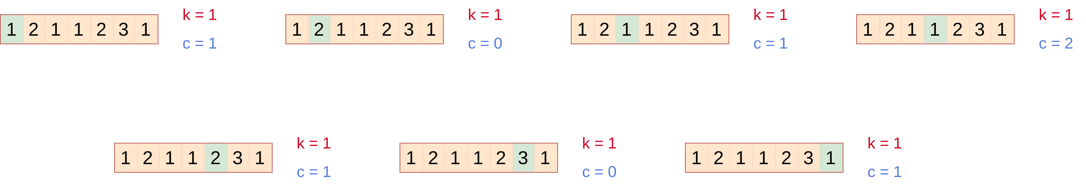
We can see that after the first pass the possible majority element is the integer $1$ . If we count its frequency in the second pass, we verify that integer $1$ is the majority element.

6. Comparison of Algorithms

In the table above we summarize the time and space complexity of each algorithm:

We see that the Boyer-Moore algorithm is the best algorithm for the majority problem with $\mathbf{O(n)}$ time complexity and $\mathbf{O(1)}$ space complexity.

7. Conclusion

In this article, we talked about how to compute the majority element in a sequence. We first presented two simple approaches and discussed their drawbacks regarding space complexity. Then we presented the Boyer-Moore algorithm that runs in linear time and constant space complexity.

Full Archive

About Baeldung

Core Concepts

Operating Systems

Artificial Intelligence

Graph Theory

Latex